Reproducing the analysis in the original study is a valuable step when planning a replication.
It allows you to verify that the original analysis is correct. Minor errors are common, and occasionally the original finding does not hold up under scrutiny.
Reproduction deepens your understanding of the methodology by showing which variables were recorded and how they were used.
The reproduction often yields code that you can reuse, ensuring that your analysis will match the methods in the original paper.
Reproduction is only possible when the original data are available, either in a public repository or directly from the authors.
I start by downloading and unzipping the data file and loading the CSV for Study 3b into the R environment.
Code
# Create data directoryif (!dir.exists("data")) {dir.create("data")}# Check if data exists, if not download and unzipif (!file.exists("data/ResearchBox 379/Data/Study 3b Data.csv")) {# Download if zip doesn't existif (!file.exists("data/ResearchBox_379.zip")) {download.file("https://researchbox.org/379&PEER_REVIEW_passcode=MOQTEQ", destfile ="data/ResearchBox_379.zip") }# Unzipunzip("data/ResearchBox_379.zip", exdir ="data")}# The downloaded zip file should be placed in the 'data' folder# unzip("data/ResearchBox_379.zip", exdir = "data")# Load Study 3b datadata <-read.csv("data/ResearchBox 379/Data/Study 3b Data.csv", header =TRUE,sep =",", na.strings =".")
29.1.2 Clean variable names and labels
I then amended the variable names to make them more readable (e.g. replacing the numbers for each condition with the words they represent: 1=control, etc.) and convert them into the correct variable type (e.g. convert to factor).
I then run a quick check on the number of observations. I note from the paper that 217 participants failed attention checks, 187 did not complete enough questions to get to the dependent variable, and there was a final sample of 1036. This gives 1440 participants.
Code
# Total participantslength(data$ID)
[1] 1440
Code
# Participants who chose between the model and human forecaststable(data$modelBonus)
choseHuman choseModel
       517        519
As expected, I found 1440 participants and 517+519=1036 dependent variable observations.
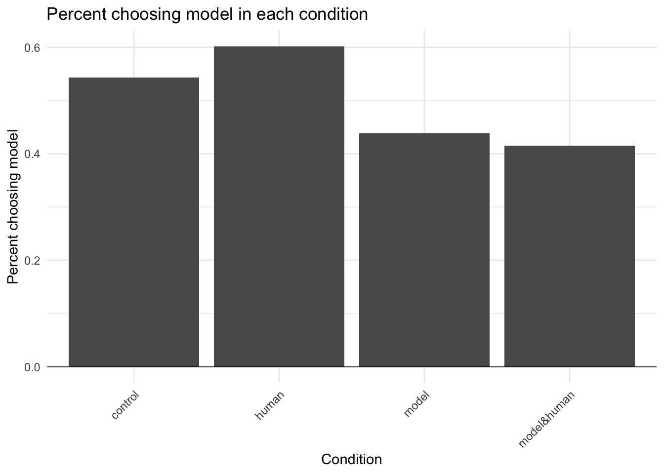
29.1.4 Choices by condition
I then broke down the dependent variable findings in more detail to see what each participant chose (human or model) in each condition.
Code
# Choice countstbl <-table(data$modelBonus, data$condition)tbl <-rbind(tbl, total =colSums(tbl))tbl
           control human model model&human
choseHuman     122   104   142         149
choseModel     145   157   111         106
total          267   261   253         255
29.1.5 Chi-squared tests
Two chi-squared tests replicate the results shown in Figure 3 of the paper. The first was a test of whether there was a difference between the two conditions without the model and the two conditions with the model. This is a test of the core hypothesis.
Code
# Compare conditions without vs. with the modelchisq.test(table(data$modelBonus, data$model), correct =FALSE)
The second was a test of whether there was a difference between the two conditions without and the two conditions with the human experience. This test was run to see whether the experience of seeing their own errors changed the participants’ choices.
Code
# Compare conditions without vs. with the human experiencechisq.test(table(data$modelBonus, data$human), correct =FALSE)
Finally, I replicate the analysis related to Study 1 as shown in Table 3. The table includes several elements:
A t-test of whether the bonus would have been higher if the model was chosen rather than the human
A t-test of whether the average absolute error was higher for the model or human in the Stage 1 unincentivised forecasts
A t-test of whether the average absolute error was higher for the model or human in the Stage 3 incentivised forecasts
The code generates the numbers required to fill the table.
Code
# Calculate human and model mean rewards m <-round(mean(data$bonusFromModel, na.rm=TRUE), 2)h <-round(mean(data$bonusFromHuman, na.rm=TRUE), 2)# Bonus if chose model vs. humanbonusModel <-t.test(data$bonusFromModel, data$bonusFromHuman, paired=TRUE)p <-signif(bonusModel$p.value, 2)t <-round(bonusModel$statistic, 2)d <-round(bonusModel$estimate, 2)# Participants' AAE compared to model's AAE for stage 1 forecastsstage1AAE <-t.test(data$humanAAE1, data$modelAAE1, paired=TRUE)p1 <-signif(stage1AAE$p.value, 2)t1 <-round(stage1AAE$statistic, 2)d1 <-round(stage1AAE$estimate, 2)AAEm <-round(mean(data[data$condition=='model&human', 'modelAAE1'], na.rm=TRUE), 2)AAEh <-round(mean(data[data$condition=='model&human', 'humanAAE1'], na.rm=TRUE), 2)# Participants' AAE compared to model's AAE for stage 2 forecastsstage2AAE <-t.test(data$humanAAE2, data$modelAAE2, paired=TRUE)p2 <-signif(stage2AAE$p.value, 2)t2 <-round(stage2AAE$statistic, 2)d2 <-round(stage2AAE$estimate, 2)AAEm2 <-round(mean(data$modelAAE2, na.rm=TRUE), 2)AAEh2 <-round(mean(data$humanAAE2, na.rm=TRUE), 2)
Table 3 results
Model
Human
Difference
t score
p value
Bonus
$0.49
$0.3
$0.2
14.4
5.8^{-43}
Stage 1 error
4.39
8.32
3.93
17.3
6.2^{-45}
Stage 2 error
4.32
8.34
4.03
15.44
1.5^{-48}
The numbers match those provided in the paper.
29.1.8 Statcheck
The above analysis relates to Study 3b only. While I won’t reproduce the other results from the paper, one quick robustness check can be performed using statcheck. To use statcheck, you upload a pdf, HTML or docx of the paper. Statcheck then extracts details of the tests reported in the paper and checks that the reported numbers are consistent. (There is also an R package for statcheck allowing you to run your own statcheck implementation.)
I uploaded the Dietvorst et al (2015) pdf, but the analysis did not work. I then accessed a HTML download of the paper using the UTS library website. Uploading the HTML version of the paper resulted in the following.