Power is the probability that you will reject the null hypothesis when it is false. Power is a function of the significance level, the effect size and the sample size.
The stricter the significance level you use in your experiment, the lower the power of the experiment. As you decrease the probability of false positives by using a more stringent significance level, you also reduce the probability of true positives.
The larger and the less variable the effect size, the more power the experiment has to detect an effect. A highly variable effect has a higher probability of getting an extreme result that generates an error.
Increasing the sample size reduces the standard error of your estimated effect size. If the alternative hypothesis is true, you will have a greater probability of detecting an effect of any given size.
30.2 Power analysis
A power analysis is an assessment of the power of a study. You can use power analysis to determine the sample size required to detect a given effect size with a given significance level. You can also use it to assess the power of a study given the sample and effect size.
For our replication, power analysis is required to assess the paper to be replicated and to prepare for the replication. The power analysis will help us to answer the following questions:
What was the probability that the original study would have found an effect under reasonable assumptions as to the size of the effect? If the study is underpowered, this is grounds to question whether we are seeing the full universe of studies or whether we are seeing a study unrepresentative of what we would expect in a replication.
How many participants do we need to recruit to have a reasonable chance of replicating the effect?
We first run a power analysis using data from the original experiment. You should not use post-experiment power analysis to justify the sample size in the original study, as any significant effect in an underpowered study is likely to be exaggerated in magnitude. If you then use this outsized effect to calculate power, it may give the impression that the experiment was adequately powered.
However, this post-experiment analysis may still provide some information about the study’s robustness. It also provides a starting point for further analysis where we adjust the effect size within a plausible range to test how sensitive the assessment of power is to the effect size.
To calculate power, we need to know the sample size (per group) and the proportion choosing the model in each group.
30.2.1 Class example
In (Dietvorst et al., 2015) Study 3b, the smallest group for the main hypothesis test had 508 members (253 model plus 255 model and human).
I will use the R command power.prop.test and G*Power to do these calculations.
30.2.1.1 R
power.prop.test requires that we provide all except one of the number of observations per group (n), the probability in one group (p1), the probability in the other group (p2), the power of the test and the significance level. The function then calculates the left-out parameter.
power.prop.test only allows one group size, so you should use the smallest.
The power of that comparison is:
Code
power.prop.test(n=508, p1=302/528, p2=217/508)
     Two-sample comparison of proportions power calculation

              n = 508
             p1 = 0.5719697
             p2 = 0.4271654
      sig.level = 0.05
          power = 0.9963619
    alternative = two.sided

NOTE: n is number in *each* group
The power of the test was over 99%.
If I wished to calculate the power using the size of both groups (including the larger group will marginally increase power - in this case the control and human groups combined had 528 participants), you can use the pwr.2p.test from the pwr package. In this function, h is the effect size.
Code
# Load the pwr packagelibrary(pwr)# Perform the power testpwr.2p2n.test(h =ES.h(p1 =302/528, p2 =217/508), n1 =528,n2 =508,sig.level =0.05,power =NULL,alternative ="two.sided" )
     difference of proportion power calculation for binomial distribution (arcsine transformation)

              h = 0.2906306
             n1 = 528
             n2 = 508
      sig.level = 0.05
          power = 0.9967004
    alternative = two.sided

NOTE: different sample sizes
We can see that the power of the test was over 99% (and calculated as being marginally higher than that for the first test).
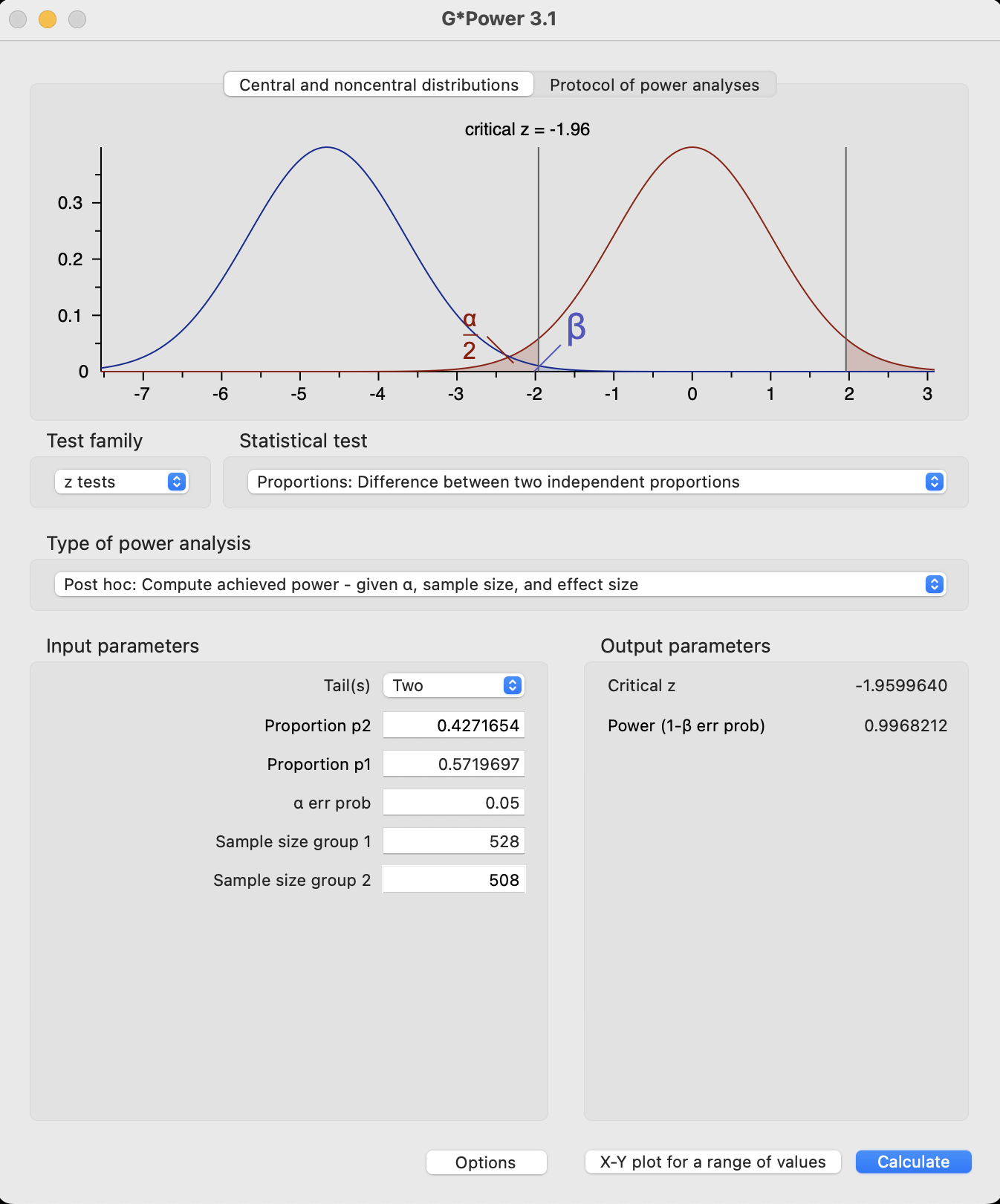
30.2.1.2 G*Power
We can also calculate power in G*Power.
In G*Power, we select the type of test that was conducted (z-test, difference between two independent proportions) and select the analysis as a post hoc calculation of achieved power. Pressing calculate gives us the result and a graph of the distributions.
30.2.1.3 Realistic effect sizes
As noted above, we should not simply take the effect size from the original study and use it to calculate power. We should also look at other studies to see what a reasonable effect size might be. We can then calculate power for a range of effect sizes.
The effect size in Study 3a of (Dietvorst et al., 2015) was 16%, with 57% in the control and 41% in the model group choosing the model. This is a similar size to the effect size in Study 3b.
Similarly, (Jung and Seiter, 2021) found that 67% of the control group and 47% of the treatment group chose the model in their replication of Study 3b. This effect size is larger than in Study 3b of (Dietvorst et al., 2015).
On that basis, the above power calculations may be a fair calcation of the power of the test.
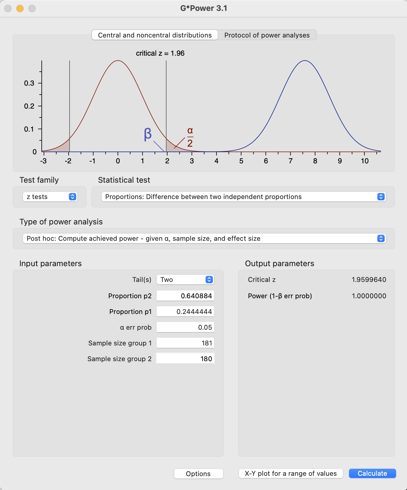
An illustration of the danger of taking the effect size in the experiment on face value involves Study 1 of (Dietvorst et al., 2015). In Study 1, the smallest comparison group had 180 members (90 in the model and 90 in the model and human groups). The control and human conditions had 116 of 181 choose the model, and the model conditions had 44 of 180 choose the model. The power of that comparison was:
Code
power.prop.test(n=180, p1=116/181, p2=44/180)
     Two-sample comparison of proportions power calculation

              n = 180
             p1 = 0.640884
             p2 = 0.2444444
      sig.level = 0.05
          power = 1
    alternative = two.sided

NOTE: n is number in *each* group
NoteG*Power
The post-experiment calculation of the power of the test is effectively 100%.
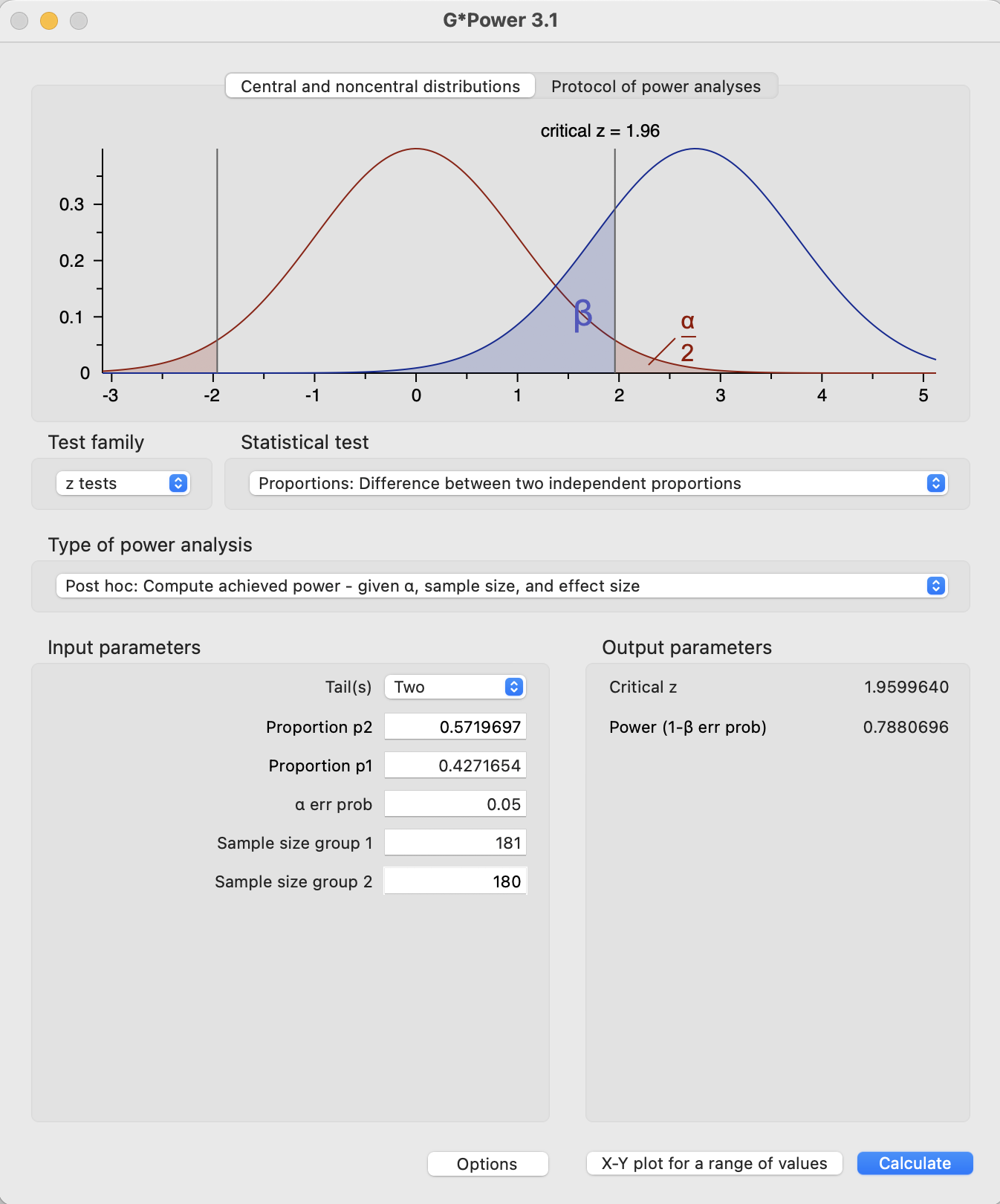
However, assuming the true effect size in Study 1 is closer to that in Study 3b, we would have the following power.
Code
power.prop.test(n=180, p1=302/528, p2=217/508)
     Two-sample comparison of proportions power calculation

              n = 180
             p1 = 0.5719697
             p2 = 0.4271654
      sig.level = 0.05
          power = 0.7869534
    alternative = two.sided

NOTE: n is number in *each* group
NoteG*Power
If that effect size was the true effect size, that gives 78% power, which is below the common rule of thumb of 80% power and substantially below a better target of 90%.
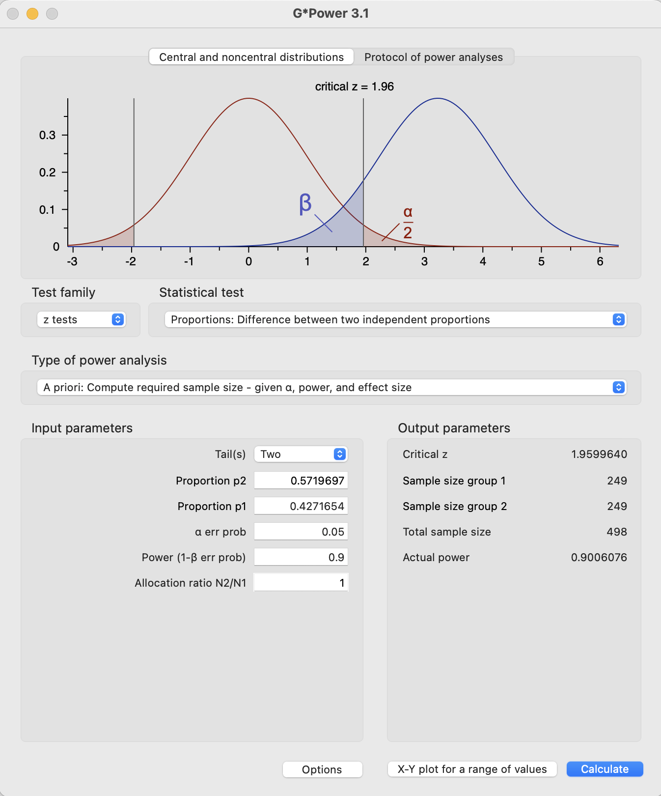
For caution, let us assume that the smallest effect size, that in Dietvorst et al (2015) Study 3b is representative of the true effect size for Study 1. We can then calculate the sample size required to achieve 90% power as:
     Two-sample comparison of proportions power calculation

              n = 248.471
             p1 = 0.5719697
             p2 = 0.4271654
      sig.level = 0.05
          power = 0.9
    alternative = two.sided

NOTE: n is number in *each* group
NoteG*Power
Ninety per cent power would require a sample of 249 in each combined group.
The above is as much art as science but gives a feel for the reasonable sample size. I would suggest a sample size of at least 250 for each group (500 in the combined groups), as was used in the original study, is adequate for replicating Study 3b. If I were replicating Study 1, I would likely use a larger sample than that used by Dietvorst et al.
30.3 An example of an underpowered study
(Kanazawa, 2007) tested the hypothesis that physically attractive parents have more daughters (as a test of the Trivers-Willard hypothesis). He found that 44% of children to parents rated “very attractive” were sons, compared to 52% for other parents.
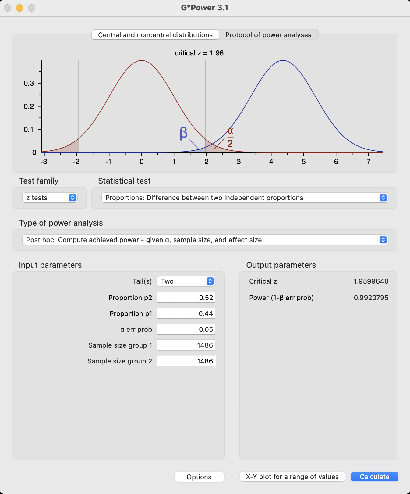
A total sample of 2972 children was available for the analysis. Assuming two equal-size groups (which will tend to inflate our estimate of power), the post-experiment analysis of power is as follows.
Code
power.prop.test(n=1486, p1=0.52, p2=0.44)
     Two-sample comparison of proportions power calculation

              n = 1486
             p1 = 0.52
             p2 = 0.44
      sig.level = 0.05
          power = 0.9920795
    alternative = two.sided

NOTE: n is number in *each* group
NoteG*Power
Based on analysis of the experiment itself, the study seems well-powered. But what if the effect size was exaggerated in magnitude?
(Gelman and Weakliem, 2009) looked to the broader literature to see what a reasonable effect size might be. They write.
There is a large literature on variation in the sex ratio of human births, and the effects that have been found have been on the order of 1 percentage point (for example, the probability of a girl birth shifting from 48.5 percent to 49.5 percent). Variation attributable to factors such as race, parental age, birth order, maternal weight, partnership status and season of birth is estimated at from less than 0.3 percentage points to about 2 percentage points, with larger changes (as high as 3 percentage points) arising under economic conditions of poverty and famine. That extreme deprivation increases the proportion of girl births is no surprise, given reliable findings that male fetuses (and also male babies and adults) are more likely than females to die under adverse conditions. Based on our literature review, we would expect any effects of beauty on the sex ratio to be less than 1 percentage point, which represents the range of natural variation under normal conditions.
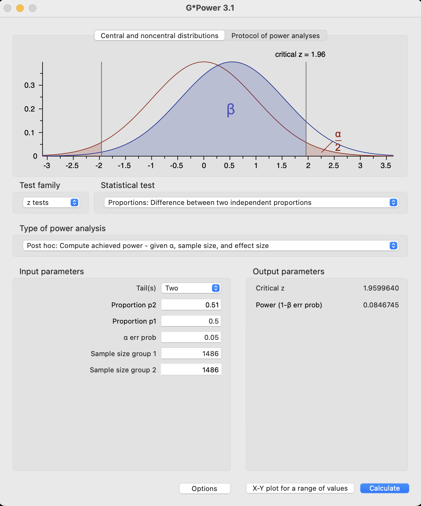
If we wanted to test a more reasonable effect size, in this case 0.3% and 1%, we get the following power.
Code
power.prop.test(n=1486, p1=0.51, p2=0.5)
     Two-sample comparison of proportions power calculation

              n = 1486
             p1 = 0.51
             p2 = 0.5
      sig.level = 0.05
          power = 0.07855669
    alternative = two.sided

NOTE: n is number in *each* group
NoteG*Power
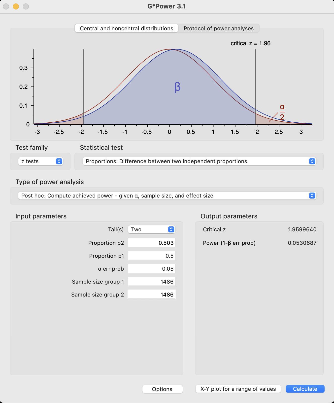
Code
power.prop.test(n=1486, p1=0.503, p2=0.5)
     Two-sample comparison of proportions power calculation

              n = 1486
             p1 = 0.503
             p2 = 0.5
      sig.level = 0.05
          power = 0.03621362
    alternative = two.sided

NOTE: n is number in *each* group
NoteG*Power
A more reasonable effect size leads to power between 3.6 and 7.8%.
Note that the G*Power and R power.prop.test results are similar but not identical at low power. The R test is more conservative at low power as it does not include in the power the probability of rejection in the opposite direction of the true effect. You can get the same result in R by setting strict=TRUE.
If we wanted to replicate the result in a new sample, we would want a much larger sample. How much larger?
Code
power.prop.test(p1=0.51, p2=0.5, power=0.8)
     Two-sample comparison of proportions power calculation

              n = 39239.3
             p1 = 0.51
             p2 = 0.5
      sig.level = 0.05
          power = 0.8
    alternative = two.sided

NOTE: n is number in *each* group
NoteG*Power
Code
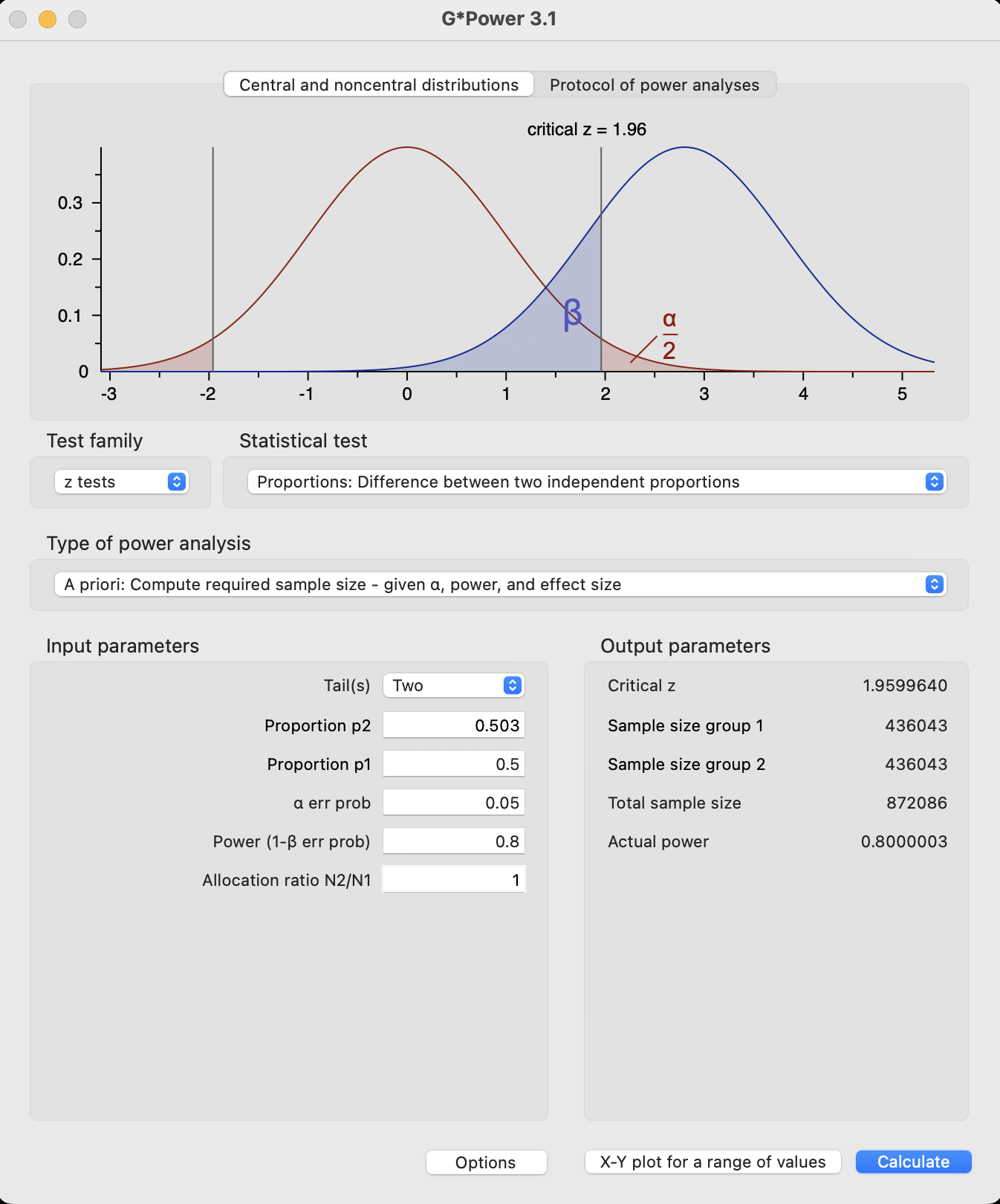
power.prop.test(p1=0.503, p2=0.5, power=0.8)
     Two-sample comparison of proportions power calculation

              n = 436043.8
             p1 = 0.503
             p2 = 0.5
      sig.level = 0.05
          power = 0.8
    alternative = two.sided

NOTE: n is number in *each* group
NoteG*Power
For 80% power, we would need over 40,000 people for a 1% effect size and over 400,000 for a 0.3% effect size. The original study appears grossly underpowered for the effect the author designed it to detect. A replication should use a sample size closer to 400,000 people than the original study’s 2972.
Dietvorst, B. J., Simmons, J. P., and Massey, C. (2015). Algorithm aversion: People erroneously avoid algorithms after seeing them err. Journal of Experimental Psychology: General, 144, 114–126. https://doi.org/10.1037/xge0000033
Gelman, A., and Weakliem, D. (2009). What is the probability that a Republican will be elected president in 2008? American Scientist, 97(2), 110–116.
Jung, M., and Seiter, M. (2021). Towards a better understanding on mitigating algorithm aversion in forecasting: an experimental study. Journal of Management Control, 32(4), 495–516. https://doi.org/10.1007/s00187-021-00326-3
Kanazawa, S. (2007). Beautiful parents have more daughters: A further implication of the generalized trivers-willard hypothesis (the “beauty premium” is a feature of humankind). Journal of Theoretical Biology, 244(1), 133–140. https://doi.org/10.1016/j.jtbi.2006.07.017